Introduction to Neural Networks and Deep Learning

The simplest definition of a neural network, more properly referred to as an 'artificial' neural network (ANN), is provided by the inventor of one of the first neurocomputers, Dr. Robert Hecht-Nielson. He defines a neural network as:

a computing system made up of a number of simple, highly interconnected processing elements, which process information by their dynamic state response to external inputs.

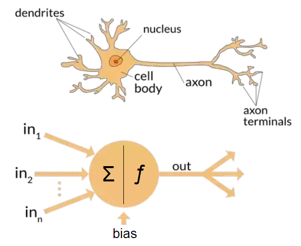
Simple Processing Element

This is a neuron.

Dynamic response

Two parts:

• $s$, which is a weighted sum of the inputs, $s = \sum \overrightarrow{w} \cdot \overrightarrow{x}$
• $f(s)$

For a linear model: $f(s) = s$. For a non-linear model, $f(s)$ will apply a transformation.

Examples:

• Logistic curve
• tanh
• ReLU Activation Function
• Step Function

Neural Networks as Supervised Learners

Can be used for regression or classification

• classification: Bike, Drive
• Regression: # of km

Learning as an Optimization Problem

The model learned should MINIMIZE the error on the overall training set.

Understanding Different Errors

Context: Tourist agency would like to figure out what is the best duration for excursions.

Training: Data with a single feature: 1,6,6,2,1,6,3,6,4,6,6

Model 1: Take the most common value in dataset. Model always predict 6 as preferred time.

Model 2: Rounded Average 47/11 = 4.27 = 4. Model always predicts 4 (average time).

L1 Error

$L_1 (E) = \sum_{e\in E} |o_e-p_e|$

Test: new people are asked about their preferences, and this data is gathered: {2,3,6,6,3,5}.

L1 Error Basically looks at difference between predictions and sums it.

L2 Error

$L_2 (E) = 1/2 \sum_{e\in E} (o_e-p_e)^2$

Now L2 Error looks at difference between predictions squared and sums and divided by half.

L(infinite) Error

$L_\infty (E) = \mathrm{max}_{e\in E} (o_e-p_e)$

Picks the max error out of all the errors

How to Minimize Error?

Greedy Algorithm: Gradient Descent

Let's evaluate the contribution of a weight on the error, and adjust that weight(up or down) to reduce the error.

$\frac{dE}{dw_i}$, we take the derivate of the error according to the weight.

Advantage of L2:

• if gradient(derivative) is positive, bring down
• if gradient is negative, bring up

Disadvantage of L1:

• there is discontinuity at some points.

Linear Regression Learner

• gradient descent for linear regression

Gradient Descent

1. Initialize weights at random
2. Repeat
   • For each example in the training set:
     1. Predict $\hat{y}$ (forward pass)
     2. Calculate $\delta = -(y-\hat{y})$
     3. For each weight $w_i$
        • Calculate derivate of error $\frac{dE}{dw_i} = \delta x_i$
        • Update weight $w_i^{(t)} = w_i^{(t-1)}-\alpha \frac{dE}{dw_i}$
3. Until "done"
   • Fixed number of iterations
   • Error < error threshold
   • $w_i (t+1) - w_i(t)$ < change threshold

Normalization

before starting the learning, we can normalize (between -1 and 1) or between (0 and 1) each of the attributes.

Logistic Regression Learner

$\hat{y} = f(s) = \frac{1}{1+e^{-s}}$ -> formula of sigmoid function.

This is known as a perceptron as it is a non-linear function.

Gradient Descent

1. Initialize weights at random
2. Repeat
   • For each example in the training set:
     1. Predict $\hat{y}$ (forward pass)
     2. For each weight $w_i$
        • Calculate derivate of error $\frac{dE}{dw_i}$
        • Update weight $w_i^{(t)} = w_i^{(t-1)}-\alpha \frac{dE}{dw_i}$
3. Until "done"
   • Fixed number of iterations
   • Error < error threshold
   • $w_i (t+1) - w_i(t)$ < change threshold

Log Loss Error

To optimize the log loss error for logistic regression, minimize the negative log-likelihood.

$LL(E, w) = - (\sum_{e \in E} (Y(e) * \log{\hat{Y}} (e) + (1-Y(e))*\log{(1-\hat{Y}(e))}))$

where $\hat{Y}$ is the sigmoid function.

Multinomial Perceptron

Expansion to Multiple Mutually Exclusive Classes leads to a multinomial perceptron.

Linearity

$s_j = \sum_{i=0}^n w_{ij} \cdot x_i$

Non-Linearity

Assume m classes. Instead of the sigmoid, now the output on node $k$ (class k), among the m node, is given by the softmax equation:

$o_k = \frac{e^s k}{\sum_{j=1}^m e^s j}$

Error Function

The error can still be the cross-entropy, generalized to multiple classes, given by:

$E(t,o) = - \sum_{j=1}^m t_j \cdot \log{o_j}$

where $t_j$ is the target(0,1) and $o_j$ is the output.

Gradient Descent

1. Initialize weights at random
2. Repeat
   • For each example in the training set:
     1. Predict $\hat{y}$ (forward pass)
     2. For each weight $w_i$
        • Calculate derivate of error $\frac{dE}{dw_i}$
        • Update weight $w_i^{(t)} = w_i^{(t-1)}-\alpha \frac{dE}{dw_i}$
3. Until "done"
   • Fixed number of iterations
   • Error < error threshold
   • $w_i (t+1) - w_i(t)$ < change threshold

XOR Affair

Limit to linear Separators

• there is no way to draw a single straight line so that the circles are on one of the line and the dots on the other side.
• Perceptron is unable to find a line separating even parity input patterns from odd parity input patterns.

Adding a Layer

Solution to XOR problem is to add a layer.