Statistical Inference

One of the goals of statistical inference to draw conclusions about a population based on a random sample from the population.

Specifically, we seek to estimate an unknown parameter $\theta$, say using a single quantity called the point estimate $\overline{\theta}$.

The point estimate is obtained using a statistic, which is simply a function of a random sample. The probability distribution of the statistic is its sampling distribution.

Examples of a statistic include:

• sample mean and sample median
• sample variance and sample standard distribution
• sample quantiles

Estimator Variance and Standard Error

The standard error of a statistic is the standard deviation of its sampling distribution

For instance, if observations $X_1, ..., X_n$ come from a population with unknown mean $\mu$ and known variance $\sigma^2$, then $\mathrm{Var}(\overline{X}) = \sigma^2/n$ and the standard error of $\overline{X}$ is

$\sigma_{\overline{X}} = \frac{\sigma}{\sqrt{n}}$

if the variance of the original population is unknown, then it is estimated by the sample variance $S^2$ and the estimated standard error $\overline{X}$:

$\sigma_{\overline{X}} = \frac{S}{\sqrt{n}}$
$S^2 = \frac{1}{n-1}\sum_{i-1}^{n}(X_i-\overline{X})^2$

Confidence Interval

For mean When SD is known

Consider a sample ${x_1, ..., x_n}$ from a normal population with known variance $\sigma^2$ and unknown mean $\mu$. The sample mean is a point estimate of $\mu$.

$\overline{x} = \frac{x_1 + ... + x_n}{n}$

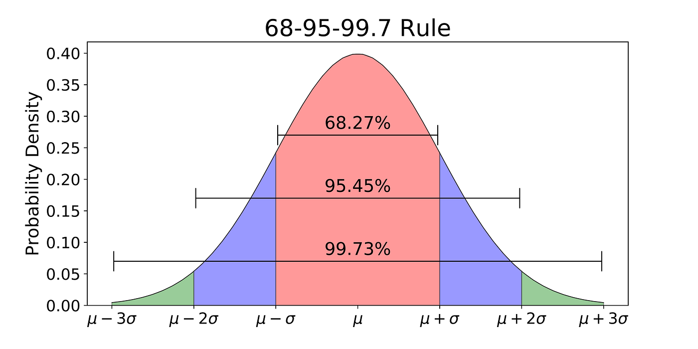
The 68-96-99.7 Rule

68% of the data is within 1 standard deviation, 95% is within 2 standard deviation, 99.7% is within 3 standard deviations.

The symmetric confidence interval for $\mu$ is

$\overline{X} - k\frac{\sigma}{\sqrt{n}} < \mu < \overline{X} + k\frac{\sigma}{\sqrt{n}} \Rightarrow \overline{X} \pm k\frac{\sigma}{\sqrt{n}}$

For mean when SD is known (reprise)

Another approach to C.I. building is to specify the proportion of the area under $φ$(z) of interest, and then to determine the critical values (the endpoints) of the interval.

For a symmetric 95% confidence interval, we need to find $z^* > 0$ such that $\mathrm{P}(-z^* < Z < z^*) ≈ 0.95$.

But the LHS can be re-written as

$\mathrm{P}(-z^* < Z < z^*) = Φ(z^*) - Φ(-z^*) = Φ(z^*) - (1 - Φ(z^*)) = 2Φ(z^*) - 1$

The confidence level 1 - α is usually expressed in terms of a small α, e.g. α = 0.05 ⇒ 1 - α = 0.95 confidence level.

For α = 0.01, 0.02, . . . , 0.98, 0.99, the corresponding $z_α$ are called the percentiles of the standard normal distribution. In general,

P$(Z > z_α) = α ⇒ z_α$ is the $100(1 - α)$ percentile

The symmetric 100(1 - α)% confidence interval can generally be written as:

$\overline{X} \pm z_{a/2}\frac{\sigma}{\sqrt{n}}$

For a given confidence level α, shorter confidence intervals are better in relation to estimating the mean:

• estimates become better when the sample size n increases;
• estimates become better when σ decreases.

Choice of Sample Size

The error we commit by estimating \mu via the sample mean X is smaller than $z_{α/2}\frac{\sigma}{\sqrt{n}}$, with probability 100(1 - α)%.

If we want to control the error, the only thing we can really do is control the sample size:

$E > z_{α/2}σ\sqrt{n} ⇒ n > (\frac{z_{α/2}σ}{E})^2$

If σ is known, we know from the CLT that $\frac{X-\mu}{σ/\sqrt{n}} \sim N (0, 1)$.

If σ is unknown, it can be shown that $\frac{X-\mu}{S/\sqrt{n}}$ follows approximately $t(n - 1)$, the Student T-distribution with $n - 1$ degrees of freedom.

Consequently, for a confidence level α,

$P(-t_{α/2}(n - 1) < \frac{X-\mu}{S/\sqrt{n}}< t_{α/2}(n - 1))≈ 1 - α$,

Equality is reached if the underlying population is normal.

$100(1 - α)$ C.I. for $\mu : \overline{X} ± t_{α/2}(n - 1) S/\sqrt{n}$.

Confidence Interval for a Proportion

If $X ∼ B(n, p)$ (number of successes in $n$ trials), then the point estimator for $p$ is $P = X/n$.

Recall that $\mathrm{E}[X] = np$ and $\mathrm{Var}[X] = np(1 - p)$.

We can standardize any random variable: $Z = \frac{X - \mu}{σ} = \frac{nP - np}{\sqrt{np(1 - p)}} = \frac{P - p}{\sqrt{p(1-p)/n}}$ is approximately $N (0, 1)$.

To calculate the confidence interval for a proportion:

$\overline{p} \pm z_{\alpha/2}\sqrt{\frac{\overline{p}(1-\overline{p})}{n}}$

Summary

Sample: ${X_1, . . . , X_n}$. Objective: predict \mu with confidence level α.

If population is normal with known variance σ2, the exact 100(1-α)% C.I. is $X ± z_{α/2}\frac{σ}{\sqrt{n}}$.

If population is non-normal with known variance $σ^2$ and $n$ is ‘big’, the approximate 100(1 - α)% C.I. is $X ± z_{α/2}\frac{σ}{\sqrt{n}}$.

If population is normal with unknown variance, the exact $100(1 - α)$ C.I. is $X ± t_{α/2}(n - 1)\frac{S}{\sqrt{n}}$.

If population has unknown variance and n is ‘big’, the approximate $100(1 - α)$ C.I. is $X ± z_{α/2}\frac{S}{\sqrt{n}}$.